# Demo: Keyword Search with Sparse Vectors
Use sparse vectors for keywords-based text retrieval.
## What You'll Learn
- Connection between Sparse Vectors & keywords-based retrieval
- Using BM25 in Qdrant
- Sparse Neural Retrieval
- Using SPLADE++ in Qdrant
## Text Encoding
In sparse vectors, each non‑zero dimension represents an object that plays a specific role for the item being represented. When we work with text, the natural choice for these objects is words.
A corpus, a finite set of texts, makes it feasible to collect every unique word and form a vocabulary. Words in the vocabulary can be ordered and enumerated, which gives us indices for sparse vectors.
### Bag-of-Words
Consider a dataset of grocery shop item descriptions in English. The vocabulary for produce can be a relatively small subset of English, ordered from “apple” to “zesty” and enumerated accordingly.
```text
Vocabulary indices (illustrative):
"cheese" -> 101
"grated" -> 151
"hard" -> 190
"mac" -> 20
"and" -> 501
```
Using the vocabulary indices, we could represent each description as a sparse vector of `(index, value)` pairs.
The value could be the **term frequency (TF)**.
**Term Frequency (TF)**
The number of times a word appears in the text.
- Description: `Grated hard cheese`
Sparse vector:
```text
[(101, 1.0), (151, 1.0), (190, 1.0)]
```
- Description: `Mac and cheese`
Sparse vector:
```text
[(20, 1.0), (101, 1.0), (501, 1.0)]
```
(Notice the shared index `101` for the word `cheese`)
- Longer description with repeated terms: `four cheese pizza for cheese lovers`
Sparse vector:
```text
[(101, 2.0), (130, 1.0), (131, 1.0), (490, 1.0), (705, 1.0)]
```
This representations are called **bag-of-words**: words are placed in a sparse vector like in a bag, without preserving order, but counting their occurrences.
## The Idea Behind Sparse Text Retrieval
If texts are represented as sparse vectors, their similarity can be computed with the **dot product**.
```text
Similarity("Grated hard cheese", "Mac and cheese") = 1.0 * 1.0 = 1.0
Similarity("Grated hard cheese", "four cheese pizza for cheese lovers")
= 1.0 * 2.0 = 2.0
```
This already hints at the idea behind a keywords-based retrieval system. We could encode all our documents as sparse vectors and retrieve & rank them based on similarity to the query.
### TF-IDF
Yet in retrieval, we care about **relevance** between documents & queries. Documents with the matching keywords to the query are probably relevant to it, yet it's not the same for every keyword, while some keywords are more important than others.
#### IDF
Some keywords are common across many documents (e.g., adjectives like `tasty` or `fresh` in the dataset of grocery shop item descriptions). Others are rare and more specific (e.g., `gorgonzola`, `mozarella`).
In the grocery corpus, the keyword `mozarella` is **more important** than `tasty` because it is **rarer**.
This importance could be expressed through **Inverse Document Frequency**.
**Inverse Document Frequency (IDF)**
A corpus-level statistic indicating how many documents contain a term. The rarer the term, the higher its IDF.
#### TF-IDF Weighting
Let's enhance each document’s bag-of-words representation by scaling each term’s frequency (TF) by its corpus-level IDF.
```text
"Grated hard cheese" =
[(101, TF("cheese") * IDF("cheese")),
(151, TF("grated") * IDF("grated")),
(190, TF("hard") * IDF("hard"))]
```
Similarity then accounts for global term importance:
```text
Similarity("cheese for pizza", "Grated hard cheese")
= 1.0 * TF("cheese") * IDF("cheese")
```
**TF‑IDF** is a simple, statistical model for keyword-based text retrieval.
#### IDF in Qdrant
Computing and maintaining per-term IDF for every term in the corpus can be annoying.
> Qdrant maintains **collection-level** IDF for sparse vectors and applies it for you during scoring.
Enable the [IDF modifier](/documentation/manage-data/indexing/index.md#idf-modifier) in the collection configuration:
```http
PUT /collections/{collection_name}
{
"sparse_vectors": {
"text": {
"modifier": "idf"
}
}
}
```
```python
from qdrant_client import QdrantClient, models
client = QdrantClient(url="http://localhost:6333")
client.create_collection(
collection_name="{collection_name}",
vectors_config={},
sparse_vectors_config={
"text": models.SparseVectorParams(
modifier=models.Modifier.IDF,
),
},
)
```
```typescript
import { QdrantClient, Schemas } from "@qdrant/js-client-rest";
const client = new QdrantClient({ host: "localhost", port: 6333 });
client.createCollection("{collection_name}", {
sparse_vectors: {
"text": {
modifier: "idf"
}
}
});
```
```rust
use qdrant_client::qdrant::{
CreateCollectionBuilder, Modifier, SparseVectorParamsBuilder, SparseVectorsConfigBuilder,
};
use qdrant_client::Qdrant;
let client = Qdrant::from_url("http://localhost:6334").build()?;
let mut sparse_vectors_config = SparseVectorsConfigBuilder::default();
sparse_vectors_config.add_named_vector_params(
"text",
SparseVectorParamsBuilder::default().modifier(Modifier::Idf),
);
client
.create_collection(
CreateCollectionBuilder::new("{collection_name}")
.sparse_vectors_config(sparse_vectors_config),
)
.await?;
```
```java
import io.qdrant.client.QdrantClient;
import io.qdrant.client.QdrantGrpcClient;
import io.qdrant.client.grpc.Collections.CreateCollection;
import io.qdrant.client.grpc.Collections.Modifier;
import io.qdrant.client.grpc.Collections.SparseVectorConfig;
import io.qdrant.client.grpc.Collections.SparseVectorParams;
QdrantClient client =
new QdrantClient(QdrantGrpcClient.newBuilder("localhost", 6334, false).build());
client
.createCollectionAsync(
CreateCollection.newBuilder()
.setCollectionName("{collection_name}")
.setSparseVectorsConfig(
SparseVectorConfig.newBuilder()
.putMap("text", SparseVectorParams.newBuilder().setModifier(Modifier.Idf).build()))
.build())
.get();
```
```csharp
using Qdrant.Client;
using Qdrant.Client.Grpc;
var client = new QdrantClient("localhost", 6334);
await client.CreateCollectionAsync(
collectionName: "{collection_name}",
sparseVectorsConfig: ("text", new SparseVectorParams {
Modifier = Modifier.Idf,
})
);
```
```go
import (
"context"
"github.com/qdrant/go-client/qdrant"
)
client, err := qdrant.NewClient(&qdrant.Config{
Host: "localhost",
Port: 6334,
})
client.CreateCollection(context.Background(), &qdrant.CreateCollection{
CollectionName: "{collection_name}",
SparseVectorsConfig: qdrant.NewSparseVectorsConfig(
map[string]*qdrant.SparseVectorParams{
"text": {
Modifier: qdrant.Modifier_Idf.Enum(),
},
}),
})
```
During retrieval, Qdrant applies the IDF component per keyword when calculating similarity scores.
## Best Matching 25 (BM25)
The **TF-IDF** model already provides a good statistical approximation of a keyword’s role in texts. What it doesn’t take into account, is that **the length of documents affects the importance of the words** used in these documents.
TF-IDF will reward longer documents simply because they have more words.
The very famous formula in information retrieval, **Best Matching 25 (BM25)**, makes several adjustments to the TF-IDF model to include document length in scoring.
### BM25 Formula
For a query \(Q\) and document \(D\):
$$
\mathrm{BM25}(Q, D) \=\ \sum_{i=1}^{N} \mathrm{IDF}(q_i)\
\frac{\mathrm{TF}(q_i, D)\(k_1 + 1)}
{\mathrm{TF}(q_i, D) + k_1\\left(1 - b + b \cdot \frac{|D|}{\mathrm{avg}_{\text{corpus}}(|D|)}\right)}
$$
Most of its components we've already introduced:
- `TF(q_i, D)`: term frequency of query word `q_i` in document `D`.
- `IDF(q_i)`: inverse document frequency of `q_i` (Qdrant can calculate and maintain this).
Additional parameters controlling document length normalization and TF saturation:
- `k_1`: controls TF saturation (how strongly extra occurrences of a query word in the document increase the score).
- `b`: controls normalization by document length, balancing `|D|` against the corpus average `avg_corpus(|D|)`.
To design BM25-based retrieval on sparse vectors, the aforementioned TF-IDF representation of documents should be updated with BM25 parameters.
Let’s see how to use the BM25 retriever in practice, in Qdrant.
### BM25 in Qdrant
**Follow along in Colab:**
The BM25 formula can be represented as follows:
$$
\text{BM25}(Q, D) = \sum_{i=1}^{n} \text{IDF}(q_i) \cdot \mathrm{function}\left(\mathrm{TF}(q_i, D), k_1, b, |D|, \mathrm{avg}_{\text{corpus}}|D|\right)
$$
Qdrant provides tooling to compute IDF on the server side.
When using any retrieval formula that includes IDF, such as BM25, in Qdrant, we no longer need to include the IDF component in the sparse document representations.
The IDF component will be applied by Qdrant automatically when computing similarity scores.
#### Create a Collection for BM25 Sparse Vectors
```python
client.create_collection(
collection_name=,
sparse_vectors_config={
"bm25_sparse_vector": models.SparseVectorParams(
modifier=models.Modifier.IDF #Inverse Document Frequency
),
},
)
```
> Once enabled, **IDF is maintained at the collection level**.
#### Create & Insert BM25-based Sparse Vectors
This leaves us with the following `values` of the documents' words:
$$
\text{BM25}(d_i) = \mathrm{function}\left(\mathrm{TF}(d_i, D), k_1, b, |D|, \mathrm{avg}_{\text{corpus}}|D|\right)
$$
The [FastEmbed](/documentation/fastembed/index.md) Qdrant library provides a way to [generate these BM25 formula-based sparse representations](https://github.com/qdrant/fastembed/blob/main/fastembed/sparse/bm25.py).
> **Update:** Since Qdrant's release [1.15.2](https://github.com/qdrant/qdrant/pull/6891), the conversion to BM25 sparse vectors happens directly in Qdrant, for all the supported Qdrant clients.
> Interface-wise, it looks the same as the local inference with FastEmbed, as we show here.
> Implementation-wise, conversion to sparse representations is also the same.
The integration between Qdrant and FastEmbed allows you to simply pass your texts and BM25 formula parameters when indexing documents to Qdrant. The conversion to sparse vectors happens under the hood.
> Don’t forget to enable the `IDF` modifier when using BM25-based sparse representations generated by FastEmbed (or since 1.15.2 by Qdrant), as they intentionally exclude this component.
```python
grocery_items_descriptions = [
"Grated hard cheese",
...
]
#Estimating the average length of documents in the corpus
avg_document_length = sum(len(description.split()) for description in grocery_items_descriptions) / len(grocery_items_descriptions)
client.upsert(
collection_name=,
points=[
models.PointStruct(
id=i,
payload={"text": description},
vector={
"bm25_sparse_vector": models.Document(
text=description,
model="Qdrant/bm25",
options={"avg_len": avg_document_length} #To pass BM25 parameters, here we're using default k & b for the BM25 formula
)
},
) for i, description in enumerate(grocery_items_descriptions)
],
)
```
#### BM25 in FastEmbed: Implementation Details
**Corpus Average Length**
Qdrant and FastEmbed do not compute $\mathrm{avg}_{\text{corpus}}|D|$ (the average document length in the corpus). You must **estimate and provide this value** as a BM25 parameter.
**Default BM25 Parameters in FastEmbed (Qdrant)**
- `k = 1.2`
- `b = 0.75`
**Text Processing Pipeline**
FastEmbed uses the [Snowball stemmer](https://www.geeksforgeeks.org/snowball-stemmer-nlp/) to reduce words to their root or base form, and applies language-specific stop word lists (e.g., *and*, *or* in English) to reduce vocabulary size and improve retrieval quality.
> If you're using BM25 with Qdrant (since 1.15.2 release), you can customize stopwords lists.
#### Lexical Retrieval with BM25 & Qdrant
Now let's test our BM25-based lexical search in Qdrant.
Suppose we're searching for the word **"cheese"** — this is our query.
```python
client.query_points(
collection_name=,
using="bm25_sparse_vector",
limit=3,
query=models.Document(
text="cheese",
model="Qdrant/bm25"
),
with_vectors=True,
)
```
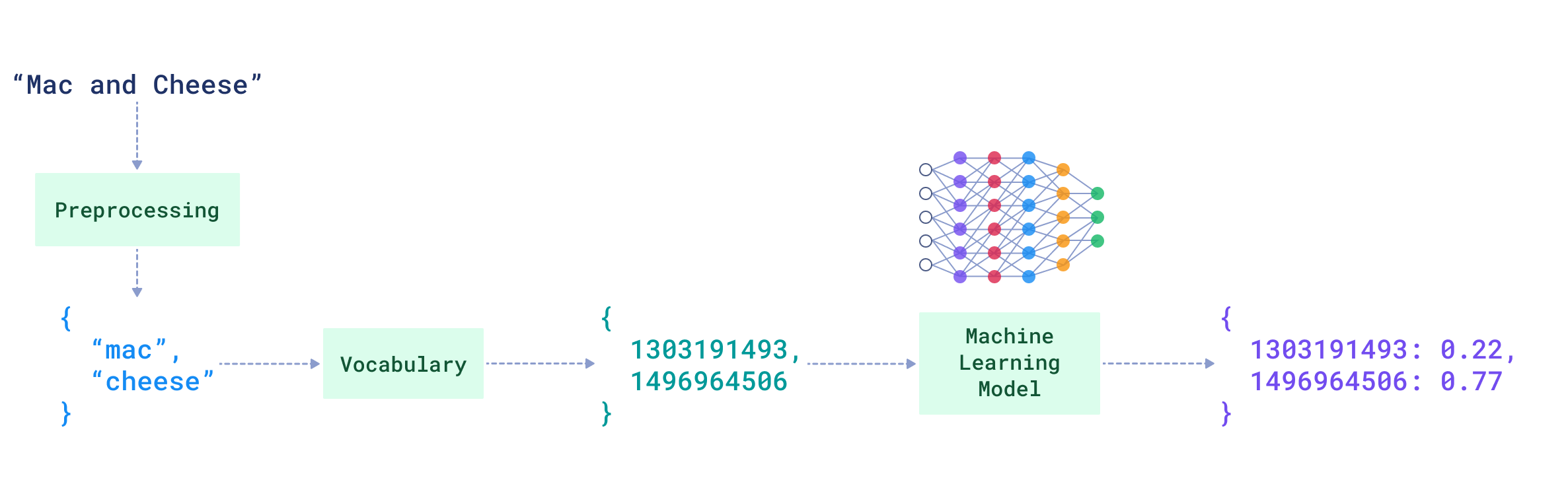
Let's break down what happens with this query and the documents indexed to Qdrant in the previous step.
**Step 1**
For every keyword in the query that is not a stop word in the target language (in our case, English, and **"cheese"** is not a stop word):
- FastEmbed (Qdrant) extracts the **stem** (root/base form) of the word.
- `"cheese"` becomes `"chees"`
- The stem is then mapped to a corresponding **index** from the vocabulary.
- `"chees"` -> `1496964506`
**Step 2**
Qdrant lookups up this keyword index (`1496964506`) in the **inverted index**, introduced in the previous video.
For every document (found via the inverted index) that contains the keyword `"cheese"`, we have the BM25-based score for `"cheese"` in that particular document, precomputed by FastEmbed (Qdrant) and stored:
$$
\mathrm{function}\left(\mathrm{TF}(\text{"cheese"}, D), k_1, b, |D|, \mathrm{avg}_{\text{corpus}}|D|\right)
$$
**Step 3**
Qdrant scales this document-specific score by the **IDF** of the keyword `"cheese"`, calculated across the entire corpus:
$$
\text{IDF}(\text{"cheese"}) \cdot \mathrm{function}\left(\mathrm{TF}(\text{"cheese"}, D), k_1, b, |D|, \mathrm{avg}_{\text{corpus}}|D|\right)
$$
**Step 4**
The final similarity score between the query and a document is the **sum of the scores of all matching keywords**:
$$
\text{BM25}(\text{"cheese"}, D) = \sum_{i=1}^{1} \text{IDF}(\text{"cheese"}) \cdot \mathrm{function}\left(\mathrm{TF}(\text{"cheese"}, D), k_1, b, |D|, \mathrm{avg}_{\text{corpus}}|D|\right)
$$
## Sparse Neural Retrieval
Now let’s explore an approach that makes keyword‑based retrieval semantically aware: **sparse neural retrieval.**
### What Does “Semantically Aware” Mean
The **bag‑of‑words** approach builds sparse text representations without word order. It counts terms, but it does not model which words appear next to which, i.e., **context**. Yet the **meaning** of a word is strongly shaped by its context.
**Example #1:**
Consider `"I want some hard-to-get cheese"` and `"I want to get some hard cheese"`. These two sentences use the same words but, due to different **word order**, put different meanings into the word `cheese.` Classical retrievers that rely on word statistics computed independently of other words cannot capture this meaning-in-context, which affects relevance.
**Example #2:**
As humans, we know that:
`"A not soft cheese"` is closer in meaning to `"hard cheese"` than to `"soft cheese"`.
**BM25** lacks this semantic awareness.
Dense retrieval might seem like the perfect solution, but in many domains **keyword‑based search** is attractive because it is **explainable**, **exact**, and **not as recall‑heavy**. The question becomes: how can we keep exact matches while making them **meaning‑aware**?
*A common pattern is to retrieve with **BM25** and then **rerank** the matched documents using a model that understands context. However, reranking **all** candidates can be expensive. It can be more efficient to make the **retriever** itself semantically aware from the start.*
### The Idea Behind Sparse Neural Retrieval
Instead of assigning word weights solely based on the corpus statistics, we could use for that **machine learning models** that have shown the ability to capture a word’s **meaning in context**.
In practice, authors of sparse neural retrievers often start from dense encoders and adapt them to produce sparse text representations: similar in shape to bag‑of‑words, but with **weights produced by a machine learning model**.
If you’re interested in details, you can check out ["Modern Sparse Neural Retrieval: From Theory to Practice"](/articles/modern-sparse-neural-retrieval/index.md) article.
Probably the most famous and used model in the field of modern sparse neural retrieval is called the Sparse Lexical and Expansion Model or SPLADE.
### SPLADE: Sparse Lexical and Expansion Model
**SPLADE** (Sparse Lexical and Expansion Model) uses bidirectional encoder representations from transformers (BERT) as a basis and, hence, is out-of-the-box mainly suitable for **English** retrieval.
SPLADE not only attempts to encode the meaning of the keywords already present in the text; it also **expands** documents and queries with **contextually fitting words**.
**Query expansion example**
```text
Q: "cheese" → ["cheese", "dairy", "food", "dish", …]
```
**Document expansion example**
```text
D: "Mac and cheese" → ["mac", "cheese", "restaurant", "brand", …]
```
This addresses the **Vocabulary Mismatch problem** when related semantically texts use different words (e.g., `hard grated cheese` vs. `parmesan`).
Qdrant and FastEmbed integration allows you to easily use one of the latest models of the SPLADE family, SPLADE++.
#### SPLADE++ in Qdrant
**Follow along in Colab:**
#### Create a Collection for Sparse Neural Retrieval with SPLADE++
SPLADE models don’t rely on corpus-level statistics like IDF to estimate word relevance. Instead, they generate term weights in sparse representations based on their interactions within the encoded text.
> Note that we’re **not configuring the Inverse Document Frequency (IDF) modifier** here, unlike in BM25-based retrieval.
```python
client.create_collection(
collection_name=,
sparse_vectors_config={
"splade_sparse_vector": models.SparseVectorParams(),
},
)
```
#### Create & Insert SPLADE++ Sparse Vectors with FastEmbed
The FastEmbed library provides **SPLADE++**; one of the latest models in the SPLADE family.
> **Update:** Since the release of [Qdrant Cloud Inference](/blog/qdrant-cloud-inference-launch/index.md), you can move SPLADE++ embedding inference from local execution (as shown in this notebook) to the Qdrant Cloud, reducing latency and centralizing resource usage.
As a result, this step looks mostly identical to using BM25 in Qdrant.
```python
grocery_items_descriptions = [
"Grated hard cheese",
"White crusty bread roll",
"Mac and cheese"
]
client.upsert(
collection_name=,
points=[
models.PointStruct(
id=i,
payload={"text": description},
vector={
"splade_sparse_vector": models.Document( #to run FastEmbed under the hood
text=description,
model="prithivida/Splade_PP_en_v1"
)
},
) for i, description in enumerate(grocery_items_descriptions)
],
)
```
However, under the hood, the process of converting a document to a sparse representation is quite different.
#### Documents to SPLADE++ Sparse Representations
SPLADE models generate sparse text representations made up of **tokens** produced by the SPLADE tokenizer.
> Tokenizers break text into smaller units called **tokens**, which form the model's **vocabulary**. Depending on the tokenizer, these tokens can be words, subwords, or even characters.
> SPLADE models operate on a fixed vocabulary of **30,522 tokens**.
#### Text to Tokens
Each document is first tokenized and the resulting tokens are mapped to their corresponding indices in the model’s vocabulary.
These indices are then used in the final sparse representation.
You can explore this process in the [Tokenizer Playground](https://huggingface.co/spaces/Xenova/the-tokenizer-playground) by selecting the `custom` tokenizer and entering `Qdrant/Splade_PP_en_v1`. For example, "*cheese*" is mapped to token index `8808`, and "*mac*" to `6097`.
#### Weighting Tokens
The tokenized text, now represented as token indices, is passed through the SPLADE model.
SPLADE **expands** the input by adding contextually relevant tokens and simultaneously assigns each token in the final sparse representation a **weight** that reflects its role in the text.
For example, "*mac and cheese*" will be expanded to: "*mac and cheese dairy apple dish & variety brand food made , foods difference eat restaurant or*", resulting in a SPLADE-generated sparse representation with **17 non-zero values**.
If you’d like to experiment with SPLADE's expansion behavior, check out our documentation on [using SPLADE in FastEmbed](/documentation/fastembed/fastembed-splade/index.md). It includes a utility function to decode SPLADE++ sparse representations back into tokens with their corresponding weights.
#### Sparse Neural Retrieval with SPLADE++ & Qdrant
Let’s now see SPLADE++ in action solving the **vocabulary mismatch** problem.
```python
client.query_points(
collection_name=,
using="splade_sparse_vector",
limit=3,
query=models.Document(
text="parmesan",
model="prithivida/Splade_PP_en_v1"
),
with_vectors=True,
)
```
SPLADE expands the query "*parmesan*" with 10+ additional tokens, making it possible to match and rank the (also expanded at indexing time) "*grated hard cheese*" as the top hit, even though "*parmesan*" doesn’t appear in any document in our dataset.
### Beyond SPLADE
SPLADE models are a strong choice for sparse neural retrieval, but they have limitations:
- **Token vs. word granularity.** SPLADE operates on **tokens** (subword pieces), which is less convenient for keyword‑oriented retrieval where users think in whole words.
```text
"Parmesan" -> "par" "##mes" "##an"
"Grated" -> "gr" "##ated"
```
This makes exact keyword reasoning and explainability harder.
- **Expansion trade‑offs.** Query/document **expansion** improves recall but can make vectors heavier and results less interpretable. For example, SPLADE++ might expand a document like `Mac and cheese` with an unrelated token such as `apple`, complicating explanation.
```text
D: "Mac and cheese" → ["mac", "cheese", "restaurant", "brand", "apple", …]
```
That said, the expansion behavior can be **fine-tuned** on domain-specific data to make it more deliberate. For example, in an e-commerce setting, fine-tuning can make SPLADE expand `mac` with `laptop` and `computer`, not `cheese`.
If you'd like to explore this direction, we walk through the full process in our 5-part series [Fine-Tuning Sparse Embeddings for E-Commerce Search](/articles/sparse-embeddings-ecommerce-part-1/index.md).
#### Qdrant's Sparse Neural Retrievers
We’ve been exploring sparse neural retrieval as a promising approach for domains where keyword-based matching is useful, but traditional methods like BM25 fall short due to their lack of semantic understanding (BM25 won't be able to distinguish "apple" in "**apple** charger" and "**apple** cutter", as opposed to sparse neural retrievers).
We’ve developed and open-sourced two custom sparse neural retrievers, both built on top of the BM25 formula, [BM42 Sparse Neural Retriever](/articles/bm42/index.md) and [miniCOIL Sparse Neural Retriever](/articles/minicoil/index.md).
Both models can be used with FastEmbed and Qdrant in the same way we demonstrated with BM25 and SPLADE++ in this tutorial.
- FastEmbed handle for **BM42**: `Qdrant/bm42-all-minilm-l6-v2-attentions`
- FastEmbed handle for **miniCOIL**: `Qdrant/minicoil-v1` (here's the detailed guide ["How to use miniCOIL"](/documentation/fastembed/fastembed-minicoil/index.md))
**miniCOIL** is the more recent of the two, and our current recommendation for new projects. It's a sparse neural retrieval model that acts as if a BM25-based retriever understood the contextual meaning of keywords and ranked results accordingly (for a query like "**apple** slicer", miniCOIL would rank "**apple** cutter" higher than "**apple** charger").
- **When to use miniCOIL:** you need **exact keyword matches** in the retrieved results, as you're working in a domain where precise term overlap matters (e.g., e-commerce, legal, medical), but want ranking to reflect the keyword's meaning in context.
- **When not to use it:** if retrieved results should be **similar by meaning** to the query but share with it no overlapping keywords. In that case, use SPLADE models or combine miniCOIL with dense vector search in a **hybrid search** setup. You'll see how to do that in the next section.
## Which Model to Choose
| | **BM25** | **miniCOIL** | **SPLADE** |
|---|---|---|---|
| **Matching** | Exact term overlap only | Exact term overlap only | Exact terms + synonym-like expansion |
| **Domain support** | High, statistical model, works out of the box on any domain | Medium-to-high, due to unsupervised learning on Web Data | Low, fine-tuning recommended |
| **Language support** | Any (tokenizer-dependent) | English (v1); vocabulary is easy to extend per-word | Typically fixed to training vocabulary (*usually BERT-based & English*) |
| **Unknown terms (not in vocabulary)** | Matched as-is (tokenizer-dependent) | Falls back to BM25 | Mapped to `[UNK]`, likely mismatched |
| **Explainability** | High | Medium-to-high | Lower without fine-tuning; expansion can introduce unrelated tokens |
| **Encoding speed** | Near-instant, tokenization only, no neural model | Medium, lightweight model | Medium-to-low, due to inner expansion mechanisms |
| **Sparse vector density** | Sparse | ~4x times less sparse than BM25 | ~8x+ times less sparse than BM25 on avg (*measured on MSMARCO*) |
| **Retrieval cost** | Low, compact sparse vectors, fast index lookup | Medium, less sparse vectors mean more computation at retrieval | High, expanded vectors are denser, increasing memory and search cost |
| **When to use** | Strong baseline; fast, lightweight, no setup required | BM25 upgrade with contextual ranking; still lightweight exact keyword matches | When synonym-like recall matters and you can invest in fine-tuning |
| **Example**: query "**apple** slicer" | Ranks "**apple** charger" and "**apple** cutter" equally as both contain "apple" | Ranks "**apple** cutter" higher, as "apple" is understood as fruit, not brand | Can match "fruit peeler" even with no keyword overlap if expansion covers it |
## Key Takeaways
- Qdrant offers sparse vectors for lexical (keyword-based) retrieval.
- Qdrant calculates **Inverse Document Frequency (IDF)** (part of BM25) on the server side. Enable it when configuring a collection with sparse vectors.
- Since 1.15.2, Qdrant supports native conversion to BM25 sparse representations.
- **Sparse neural retrieval** is keyword-based retrieval that accounts for a word’s meaning in context.
- Qdrant has its own open-sourced sparse neural retrievers (e.g., **miniCOIL**).
- When choosing a sparse retriever, lexical (e.g., BM25) or neural (e.g., SPLADE++, miniCOIL), **experiment on your data** to find the best fit.
## What's Next
Sparse retrieval, even with neural weighting, has limits when semantically similar content is expressed in very different ways. **Dense retrieval** excels at discovery and naturally bridges vocabulary mismatch.
Both methods are complementary:
- **Sparse**: precise, lightweight, explainable.
- **Dense**: flexible, strong at exploration and discovery.
Combining them yields **Hybrid Search**. See the next section for how to configure and use hybrid retrieval.