# HNSW Indexing Fundamentals
At this point, you've learned how vector search retrieves the nearest vectors to a query using cosine similarity, dot product, or Euclidean distance. How does this work at scale?
## Why Vector Search Needs Indexing
### The Vector Search Challenge
You might wonder if Qdrant calculates the distance to every single vector in your collection for each query. This method, known as brute force search, technically works but with millions or billions of vectors this is too slow per query.
Fortunately, Qdrant speeds things up with **[HNSW — Hierarchical Navigable Small Worlds](/articles/filterable-hnsw/index.md)**.
### The Library Analogy
To understand HNSW, imagine walking into a library with millions of books, looking for a specific book based on a brief description of the content. If the books were all piled up randomly, you'd have to check every book individually to find the one that matches your description best - that's brute force. While it would eventually work, it would take forever.
But libraries aren't organized like that. They're structured to naturally guide you to the right section. You walk into a library and at the top level, you choose whether your book is in the fiction or nonfiction section. Then, you narrow it down by genre - history, science, or biography. After that, you move to more specific subcategories or alphabetical order until you reach the exact shelf where your book is located.
## How HNSW Works
### Graph Structure
HNSW works similarly by building a multi-layered graph where each vector is a node. The idea is that the graph has a hierarchical structure, where the top layer contains a smaller number of nodes that are broadly connected, and each lower layer has more nodes with increasingly specific connections.
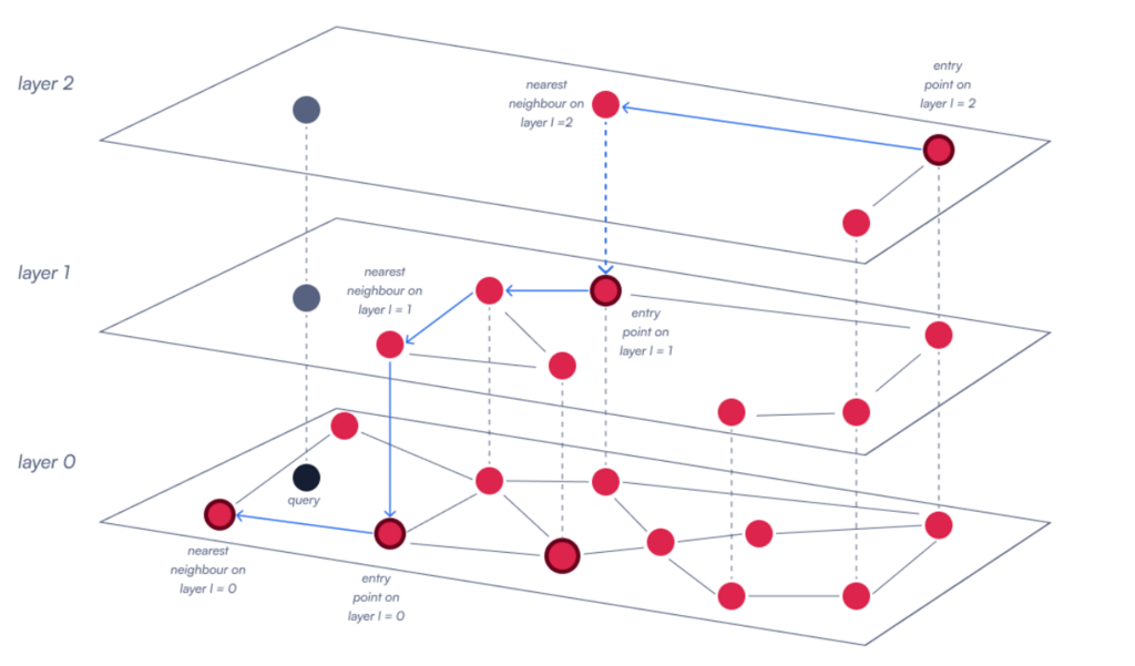
### The Search Process
When a query is performed, HNSW starts from an entry point at the top layer and navigates down through the graph, progressively moving from broader to more precise connections. At each layer, the algorithm explores the nearest neighbors of the current node to determine the best path forward. It continues this process, refining the search as it descends through the layers, until it reaches the lowest level, where it selects the final nearest neighbors.
This way, Qdrant avoids brute force and quickly narrows down the search space on large datasets.
## Configuring HNSW
We can fine-tune how our HNSW graph is built to balance search speed, accuracy, memory usage, and indexing time, depending on our use case needs. Qdrant allows you to control how the HNSW index behaves with three key parameters: `m`, `hnsw_ef`, and `ef_construct`.
### Graph Connectivity: `m`
The `m` parameter controls the maximum number of connections per node in the graph.
- Higher `m`: results in a denser graph where each vector is connected to more neighbors, which improves search accuracy because the graph has more pathways to traverse, making it less likely to miss relevant vectors. However, this also increases memory usage and indexing time since more connections must be maintained.
- Lower `m`: makes the graph sparser, reducing memory and speeding up insertion. However, search may become less accurate since fewer paths are available for traversal.
- Typical values: between 8 and 64
```python
from qdrant_client.models import HnswConfig
# Example m values
fast_config = HnswConfig(m=8, ef_construct=100, full_scan_threshold=10000) # Lower recall, less memory, faster build
balanced_config = HnswConfig(m=16, ef_construct=100, full_scan_threshold=10000) # Default - good balance
accurate_config = HnswConfig(m=32, ef_construct=100, full_scan_threshold=10000) # Better recall, more memory, slower build
```
### Build Thoroughness: `ef_construct`
The `ef_construct` parameter controls how many candidates are checked while inserting a new vector.
- Higher `ef_construct`: means more neighbors are evaluated, resulting in a more comprehensive and accurate graph. However, this also makes the indexing process slower and more computationally demanding.
- Lower `ef_construct`: speeds up the insertion process, but the graph may end up with less optimal connections, which can impact search accuracy.
- Common range: between 100 and 500. Complex data can require higher values to maintain reliable connections.
```python
# Example ef_construct values
fast_build = HnswConfig(m=16, ef_construct=100, full_scan_threshold=10000) # Default - Faster indexing, lower quality
balanced_build = HnswConfig(m=16, ef_construct=200, full_scan_threshold=10000) # Good balance
quality_build = HnswConfig(m=16, ef_construct=400, full_scan_threshold=10000) # Slower indexing, higher quality
```
### Search Thoroughness: `hnsw_ef`
The `hnsw_ef` parameter determines the number of candidates evaluated during a search query.
- Higher `hnsw_ef`: lead to more accurate search results since the algorithm explores a larger neighborhood. However, they also increase query time because more nodes are processed.
- Lower `hnsw_ef`: speed up the search but may reduce accuracy since fewer candidate vectors are considered.
- Typical range: 50–200+ depending on latency targets.
```python
from qdrant_client.models import SearchParams
# hnsw_ef is set at search time, not build time
fast_search = SearchParams(hnsw_ef=32) # Very fast, lower recall
balanced_search = SearchParams(hnsw_ef=128) # Default - good balance
accurate_search = SearchParams(hnsw_ef=256) # Higher recall, slower
```
### Parameter Summary
| Parameter | Purpose | Effect |
| ---------------- | ---------------------------- | ------------------------------------------------ |
| **m** | Links per node | Up improves recall; uses more RAM and build time |
| **ef_construct** | Candidates checked on insert | Up improves graph quality; slows indexing |
| **hnsw_ef** | Candidates checked on search | Up improves recall; slows queries |
## Choosing Settings
### Optimizing for Different Workloads
- **High-speed retrieval:** lower `m` and `hnsw_ef`; set `ef_construct` just high enough for acceptable recall.
- **Maximum recall:** raise `m`, `hnsw_ef`, and `ef_construct` and accept slower queries and builds.
- **Tight RAM:** reduce `m`; keep `ef_construct` high enough to avoid poor links.
### Memory & Indexing Behavior
Some vectors can remain unindexed depending on [optimizer](/documentation/operations/optimizer/index.md) settings e.g. when the unindexed part stays below the `indexing_threshold` (kB).
Small collections or low-dimensional vectors may not trigger HNSW indexing at all. In such cases, full-scan search (brute force) is used instead until indexing becomes beneficial
## HNSW in Action
### Why It Is Fast and Scalable
- **Sublinear Search Scaling**: Unlike O(N) brute force search, HNSW search grows roughly logarithmically with the number of vectors. This makes million-scale datasets searchable in milliseconds rather than minutes.
- **Filter‑Aware**: Qdrant extends HNSW with filter-aware indexing (Filterable HNSW), allowing fast searches under structured conditions. This avoids costly full scans when filtering by metadata.
- **Large-Scale Use**:
- Supports real-time updates while maintaining high recall
- Fits semantic search and recommendation systems
- Scales from thousands to billions of vectors
### Practical Configuration Examples
```python
from qdrant_client import QdrantClient, models
import os
client = QdrantClient(url=os.getenv("QDRANT_URL"), api_key=os.getenv("QDRANT_API_KEY"))
# For Colab:
# from google.colab import userdata
# client = QdrantClient(url=userdata.get("QDRANT_URL"), api_key=userdata.get("QDRANT_API_KEY"))
# Production configuration
client.create_collection(
collection_name="production_vectors",
vectors_config=models.VectorParams(
size=768,
distance=models.Distance.COSINE,
hnsw_config=models.HnswConfigDiff(
m=16, # Balanced connections (default)
ef_construct=200, # Good build quality (default)
full_scan_threshold=10000, # Use brute force below this size (default)
),
),
)
# Development / testing: faster builds
client.create_collection(
collection_name="dev_vectors",
vectors_config=models.VectorParams(
size=384,
distance=models.Distance.COSINE,
hnsw_config=models.HnswConfigDiff(
m=8, # Fewer connections
ef_construct=100, # Faster builds
full_scan_threshold=10000, # Use brute force below this size (default)
),
),
)
```
## Performance Benchmarking
Let's test the performance. First we upload some toy data to a new collection:
```python
import time
from qdrant_client import QdrantClient, models
import os
client = QdrantClient(url=os.getenv("QDRANT_URL"), api_key=os.getenv("QDRANT_API_KEY"))
# For Colab:
# from google.colab import userdata
# client = QdrantClient(url=userdata.get("QDRANT_URL"), api_key=userdata.get("QDRANT_API_KEY"))
collection_name = "my_collection"
if client.collection_exists(collection_name=collection_name):
client.delete_collection(collection_name=collection_name)
# Development / testing: faster builds
client.create_collection(
collection_name=collection_name,
vectors_config=models.VectorParams(
size=4,
distance=models.Distance.COSINE,
hnsw_config=models.HnswConfigDiff(
m=8, # Fewer connections
ef_construct=100, # Faster builds
full_scan_threshold=0, # Always use HNSW search, never fall back to brute force
),
),
optimizers_config=models.OptimizersConfigDiff(
indexing_threshold=100, # Low threshold to force HNSW index build on small data
),
)
# upload data
import random
points = []
for i in range(20000):
points.append(
models.PointStruct(id=i, vector=[random.random() for _ in range(4)], payload={})
)
client.upload_points(
collection_name=collection_name,
points=points,
)
```
### Search Performance
This simple local benchmark, intended as a toy example, since this approach does not take into account other factors, such as network speed.
```python
def benchmark_search_performance(collection_name, test_queries, ef_values):
"""Compare latency across hnsw_ef values"""
results = {}
for hnsw_ef in ef_values:
start_time = time.time()
for query in test_queries:
client.query_points(
collection_name=collection_name,
query=query,
limit=10,
search_params=models.SearchParams(hnsw_ef=hnsw_ef),
)
avg_time = (time.time() - start_time) / len(test_queries)
results[hnsw_ef] = avg_time
print(f"hnsw_ef={hnsw_ef}: {avg_time:.3f}s per query")
return results
# Test different hnsw_ef values
test_queries = [
[30, 60, 90, 120],
[150, 180, 210, 240],
[270, 300, 330, 360],
[390, 420, 450, 480],
[510, 540, 570, 600],
]
ef_values = [32, 64, 128, 256]
performance = benchmark_search_performance(collection_name, test_queries, ef_values)
```
### Inspecting Performance and Index Use
Use [`get_collection`](https://api.qdrant.tech/api-reference/collections/get-collection) to inspect your collection. It returns current statistics and configuration of the collection like `points_count`, `indexed_vectors_count` or `hnsw_config`. It also lists `payload_schema` for payload indexes you created.
To see whether your data is actually indexed, you need to check two things: the number of indexed vectors and the collection's status. If `indexed_vectors_count` is low, indexing may not have completed. More importantly, you should check the collection `status`. A `YELLOW` status means optimization (indexing) is still in progress, while a `GREEN` status confirms it is complete and ready for optimal performance.
If queries feel slow check:
- whether filter fields have [payload indexes](/documentation/manage-data/indexing/index.md#payload-index).
- if the payload indexes have been set before building the HNSW graph (HNSW graph building begins when you switch from `m = 0` to `m > 0`)
- if `hnsw_config.full_scan_threshold` is too high.
```python
# Inspect collection status
info = client.get_collection(collection_name)
vectors_per_point = 1 # set per your vectors_config
vectors_count = info.points_count * vectors_per_point
print(f"Collection status: {info.status}")
print(f"Total points: {info.points_count}")
print(f"Indexed vectors: {info.indexed_vectors_count}")
if vectors_count:
proportion_unindexed = 1 - (info.indexed_vectors_count / vectors_count)
else:
proportion_unindexed = 0
print(f"Proportion unindexed: {proportion_unindexed:.2%}")
if info.status == models.CollectionStatus.GREEN:
print("\n✅ Collection is indexed and ready!")
elif info.status == models.CollectionStatus.YELLOW:
print("\n⚠️ Collection is still being indexed (optimizing).")
else:
print(f"\n❌ Collection status is {info.status}.")
```
## When Not to Use HNSW
### Small Collections
For collections with fewer than 10,000 vectors, brute force is often faster and uses less RAM than building HNSW.
### Exact Search Requirements
HNSW is approximate. If you need exact results, use brute force.
### Extreme Memory Constraints
For very tight RAM budgets consider these solutions:
- **Lower `m`**: HNSW uses additional memory proportional to `m × vectors_count`.
- **Vector quantization (VQ):**
- Scalar quantization (SQ) often cuts RAM ~4×
- Binary quantization (BQ) compresses to 1‑bit per dimension and can cut RAM by large factors.
- **On Disk Storage**: Set `on_disk=true` for vectors and the HNSW index to use mmap files where only the most frequently accessed vectors are cached in RAM.
- **Disable HNSW for Reranking Embeddings:** Useful since reranking vectors such as multi‑vectors are large.
## Key Takeaways
1. **HNSW**: reduces O(N) scans to roughly O(log N) graph search
2. **`m`**: controls graph density - more connections improve accuracy but use more memory
3. **`ef_construct`**: affects graph quality - higher values create more granular graphs but take longer to build
4. **`hnsw_ef`**: controls search thoroughness - tune at query time for the speed/accuracy trade-off you need
5. **`indexed_vectors_count`**: track to confirm HNSW indexing
## What's Next
Now you understand how HNSW makes vector search fast and scalable. Next we'll combine fast search with complex filters using Qdrant’s filter‑aware HNSW.
Learn more: [HNSW in Qdrant Documentation](/documentation/manage-data/indexing/index.md#vector-index)
Ready to see how HNSW handles real-world filtering scenarios? Let's continue!